


A really accurate quartic
equation solver
This web page describes a new quartic
(4th degree) equation solver, which achieves the
theoretically attainable accuracy in its solutions.
Solutions to the quartic equation are known for
centuries already, but naively using those solutions in
computer programs leads to very inaccurate results in
many cases.
First, by using the well-known standard solution of a
quadratic equation, it is demonstrated what type of
issues can appear in computer programs, which naively
implement mathematical formulas. Although the
mathematical formulas are correct, the implementation
may suffer severe inaccuracies, due to limited precision
of the used computer arithmetic.
For a quadratic equation, it is fairly easy (but not
trivial for most people) to solve the issue of
inaccuracy in the software. For quartic equations,
however, this has proven extremely difficult. Only since
2015, with the introduction of a new analytic solution,
it is feasible to perform the full analysis, which leads
to an accurate solution in all cases.
I have performed the complete analysis for the proposed
solution of a quartic equation, and based on that
analysis I developed a software package, which can be
used to solve a general quartic equation accuracy at the
theoretically attainable accuracy, while at the same
time being very fast. On a standard CPU (e.g. core i3,
core i5 or core i7, 12th or 13th generation) it is
possible to solve 3 to 5 million quartic equations per
second per core accurately, using standard IEEE double
precision arithmetic, regardless of the given
coefficients of the quartic!
This webpage explains how accuracy can
be lost in numerical calculations, by giving an example,
and gives a short summary of the algorithm for solving
quartic equations. A full description of the algorithm
can be found in this paper: Fast robust and accurate
low-rank LDLT quartic equation solver.
There also is a software package available, both in Java
and in C. This software is available as part of a larger
set of software packages from the following page: polynomial
solver packages and utilities.
Besides code for solving quartic equations, the code
also contains high quality solvers for quadratic, cubic
and quintic equations. The solution for quadratic and
cubic equations is touched upon in the sections below,
the solution for quintic equations is based on an
efficient method, developed by Madsen and Reid in the
1970's, combined with the quartic and cubic solvers in
the same package.
![]()
Solving a quadratic equation is not
that easy!
In high school, the well-known
"abc-formula" is taught for solving a quadratic
equation.
If the equation is written as ax2 + bx + c
= 0, then, assuming a ≠ 0, the solution is
written as
![]()
Here we have the two roots of the quadratic equation.
If the number b2 −
4ac is negative, then we have two complex
roots, otherwise we have two real roots.
Now, we write a
simple computer program for solving this equation,
which has three numbers a, b, and c
as input and two numbers x1 and x2
as output. In Java, one could write the following
simple program:
package net.oelen.nummath;
public class QuadraticNaive {
// A routine to solve the equations efficiently.
// Inputs: coefficients a, b, c of the quadratic expression.
// Outputs: An array xre with at least two elements, which will
// hold the real part of the solutions and an array xim, which
// will hold the imaginary part of the two solutions.
public static void solve(double a, double b, double c,
double[] xre, double[] xim) {
double D = b*b - 4*a*c;
if (D >= 0) {
// Two real solutions.
double sq = Math.sqrt(D);
xre[0] = (-b + sq)/(2*a); xim[0] = 0.0;
xre[1] = (-b - sq)/(2*a); xim[1] = 0.0;
}
else {
// Two complex solutions.
double sq = Math.sqrt(-D);
xre[0] = -b/(2*a); xim[0] = sq/(2*a);
xre[1] = xre[0]; xim[1] = -xim[0];
}
}
// A test routine, which takes the value of a and
// two given roots and computes values for b, and c.
// a*(x-x1)*(x-x2) = a*x^2 - a*(x1+x2)*x + a*x1*x2
// ==> b = -a*(x1+x2)
// c = a*x1*x2
//
// This information, then is fed to the solver and
// the result is printed. Only real values can be
// generated with this test.
public static void test(double a, double x1, double x2) {
double b = -a*(x1+x2);
double c = a*x1*x2;
double[] xre = new double[2];
double[] xim = new double[2];
solve(a, b, c, xre, xim);
// Only print real part of solutions,
// imaginary part will always be 0.
System.out.printf("x1 = %.13e x2 = %.13e\n", xre[0], xre[1]);
}
public static void main(String[] args) {
test(1.0, 1.23456789, 9.87654321);
test(53425.7547453743573, 1.23456789, 9.87654321);
System.out.println("-----------------------");
test(1.0, 1e6, 1e-6);
test(1.0, 1e10, 1e-10);
test(1.0, -1e6, 1e-6);
System.out.println("-----------------------");
test(1.0, 1e14, -1.0);
test(7564.321541241242, 1e14, -1.0);
}
}
When the program above is compiled and
executed, then it produces the following output:
x1 = 9.8765432100000e+00 x2 = 1.2345678900000e+00
x1 = 9.8765432100000e+00 x2 = 1.2345678900000e+00
-----------------------
x1 = 1.0000000000000e+06 x2 = 1.0000076144934e-06
x1 = 1.0000000000000e+10 x2 = 0.0000000000000e+00
x1 = 1.0000076144934e-06 x2 = -1.0000000000000e+06
-----------------------
x1 = 1.0000000000000e+14 x2 = -1.0000000000000e+00
x1 = 1.0000000000000e+14 x2 = -9.9837109763591e-01
The first two lines show that the
program works nicely for the two equations with roots
equal to 1.23456789 and 9.87654321. It also demonstrates
that the roots do not depend on the factor a.
This also is as expected. If the entire equation is
multiplied with a certain number, then the roots do not
change.
The second group of three results shows less satisfactory results. The roots 106, 1010, and -106 are reproduced nicely, but the roots 10-6 and 10-10 are not reproduced well. The root 10-6 has erroneous digits after the sixth correct digit and the root 10-10 is lost completely (it is replaced by 0). In the final group of two results, the root, equal to 1014 is reproduced correctly. The first result also shows correct reproduction of the root −1, but the second test shows that the root −1 is severely corrupted, just by multiplying the equation with a constant value. Mathematically this should not change the roots, but this computer program fails miserably in this case.
![]()
Numerical cancellation
Computer systems only have limited
space for storing numbers. Modern processors, like the
Intel and AMD processors, but also the common
ARM-processors, use 64 bits of storage for one so-called
double precision floating point number. Such double
precision numbers are approximations of real
numbers. Certain real numbers, like 5⅞, 2, 1, ½, ⅛, and
¾ can be represented exactly, but others, like ⅓, ⅘ and
⅑ cannot. This is because in computers, numbers are
stored with a finite number of digits (binary digits,
just 0's and 1's). If we want to represent numbers like
⅔ with a finite number of decimal digits, then we need
to truncate, or round. E.g. when we have only 8 digits
for storing numbers, then we can write 0.66666667 as
best possible approximation of ⅔. But this number is not
exactly equal to ⅔. The numbers ⅛ and ⅒, however, can be
represented exactly as 0.12500000 and 0.10000000 in the
decimal system with 8 digits.
So, numbers in general are represented
in an inexact way in a computer system. They are rounded
to the nearest representable number. If we do
calculations with such rounded numbers, then the result
can become utterly meaningless. In the decimal system
with 8 digit approximations we give an example:
![]()
If this calculation is performed in
the 8-digit approximation system, then the result will
be quite different:
0.66666667 − 0.66666600 = 0.67000000·10-6.
Here one can see that only 2 digits of
accuracy are left in the calculation. The correct answer
in the 8-digit approximation system would be 0.66666667·10-6.
![]()
Back to the quadratic equation
Now we have the tools to understand
what happens in the solution of the quadratic equations.
The solutions are repeated here:
![]()
If you look more
carefully at these solutions, then you can see that in
the numerator two numbers are added to each other, or
subtracted from each other. Addition of two numbers of
opposite sign, or subtraction of two numbers of the
same sign can lead to catastrophic loss of accuracy,
just as demonstrated in the example above with the
8-digit approximations.
The numbers in a modern CPU have 53 binary digit
accuracy, which is appr. 16 decimal digit accuracy.
Quadratic equations, which have two real roots, where
one of the roots has a much bigger magnitude than the
other (sign does not matter), suffer from severe
numerical cancellation in one of the two solutions. If
the magnitudes of the roots are comparable (e.g. both
are numbers between 1 and 10), then the absolute
values of b and the square root are quite different
and both formulas give good results. That is the case
in the first two tests, where the roots are 1.23456789
and 9.87654321. In the case of roots, equal to 106
and 10-6, the values of b and the square
root are very close (the first 12 digits are the
same):
b ≈
-1000000.0000010000
√(b2 − 4ac)
≈ 999999.9999990000.... (up to 16 digits are given,
the ... are non-zero digits)
So, when these two numbers are added to each other
(the formula for x1), then there is
a lot of cancellation, the first 12 digits are lost!
The sum of these two is -0.0000020000.... (dots are
non-zero digits) and when this is divided by 2a
(which equals 2 in this case), then we find a root
-0.0000010000.... (non-zero digits at the dots) and we
only have 5 or 6 correct digits. For the other root x2,
the result is much better. Here the two numbers both
are negative and hence their magnitudes add up and we
keep all 16 digits precision.
What can we do
against the loss of precision in the quadratic
equation solver?
If we look at the final result of the
computer program, then things look bleak. One way is to
use more accurate computations. We need better CPU's!
Indeed, there are very special CPU's, which have 128 bit
arithmetic, and there also are software libraries, which
increase the accuracy. But these things come at a cost.
Either the hardware is much more expensive, or the
computations become much slower (a factor 5 to 10
slowdown for doubling the precision in a software
emulation may be expected).
In this particular case of the
quadratic equation solver, however, we do not need
higher precision arithmetic. Cancellation only occurs
when numbers of nearly equal magnitude and opposite sign
are added to each other or numbers of nearly equal
magnitude and same sign are subtracted from each other.
Division and multiplication do not suffer from numerical
cancellation.
If we have a quadratic equation with
roots x1 and x2,
then it can be written as
From this follows that c = a
x1 x2.
The result of the test run now looks as follows:
public static void solve(double a, double b, double c,
double[] xre, double[] xim) {
double D = b*b - 4*a*c;
if (D >= 0) {
// Two real solutions. We only compute the
// solution without cancellation by means
// of the abc-formula.
double sq = Math.sqrt(D);
if (b < 0) {
xre[0] = (-b + sq)/(2*a);
}
else {
xre[0] = (-b - sq)/(2*a);
}
xre[1] = c/(a*xre[0]);
xim[0] = xim[1] = 0.0;
}
else {
// Two complex solutions. Here we do not have
// the issue of numerical cancellation. The
// real and imaginary parts are separate numbers.
double sq = Math.sqrt(-D);
xre[0] = -b/(2*a); xim[0] = sq/(2*a);
xre[1] = xre[0]; xim[1] = -xim[0];
}
}
x1 = 9.8765432100000e+00 x2 = 1.2345678900000e+00
x1 = 9.8765432100000e+00 x2 = 1.2345678900000e+00
-----------------------
x1 = 1.0000000000000e+06 x2 = 1.0000000000000e-06
x1 = 1.0000000000000e+10 x2 = 1.0000000000000e-10
x1 = -1.0000000000000e+06 x2 = 1.0000000000000e-06
-----------------------
x1 = 1.0000000000000e+14 x2 = -1.0000000000000e+00
x1 = 1.0000000000000e+14 x2 = -1.0000000000000e+00
Here we see that all roots have excellent accuracy. The strategy of using the large magnitude-root and using that to compute the low-magnitude root has a dramatic effect! This example also demonstrates that writing computer programs for solving numerical problems needs great care and analysis. This can be quite challenging, even for only moderately complicated problems!
The code now performs much better. However, one little issue is introduced. If both b and c are equal to zero, then the code will lead to a division by 0. In code for a general library, a check will have to be added for zero coefficients. In a dedicated application this check might not be necessary, if the nature of the problem is such that b and c never will both be zero.
The above example for a quadratic equation shows what kind of subtleties can ruin the accuracy of the computed solutions and solving this requires careful mathematical analysis. For cubic equations and quartic equations, the situation is much more complicated and the analysis really is hard. A little introduction is given in the next sections.
![]()
In the 16th century, a beautiful solution for the cubic equation was discovered by Cardano and this was further polished by his student Ferrari. At that time, the concept of negative numbers was not yet fully developed and the concept of complex numbers was completely unknown, so the solutions were overly complicated for Cardano and Ferrari, using all kinds of special cases to cover the situation of three real roots, one real root, roots which are negative and roots which are positive in all kinds of combinations. In modern notation, the solution, however, is very elegant and easy to understand.
Cardano found a method for solving an equation of the form y3 + py + q = 0. Any general third degree equation ax3 + bx2 + cx + d = 0, with a ≠ 0, can be converted to this form. In order to do so, first the equation is divided by a. This does not affect the roots of the equation. The resulting equation is x3 + εx2 + φx + λ = 0, with ε = b/a, φ = c/a and λ = d/a. Next, by substituting x with (y − ⅓ ε), we get an equation in so-called depressed form y3 + py + q = 0, where p and q are fairly simple expressions in ε, φ and λ.
Cardano had the brilliant idea of replacing y by v + w. The depressed equation then becomes
(v + w)3 + p(v + w) + q = 0
After some algebraic rearrangement, this can be written as
(3vw + p)(v + w) + (v3 + w3 + q) = 0
There are no special requirements on v and w other than that v + w must be equal to y. So, one can impose an additional constraint on v and w: 3vw + p = 0. Using this constraint, expressing w as function of v leads to
w = −p / 3v and v3 − p3 / (27v3) + q = 0
By multiplying with v3 the latter equation can be transformed into a quadratic equation in v3. This equation can be solved easily and by taking the cube root, one finds a value for v. This can be used to find a value for w and hence for y = v + w. With some algebraic rearrangement, the expression for y can be written in terms of p and q as

Using x = y + ⅓ ε, one finds a solution for the original cubic equation. When p, q and ε are written in terms of the original a, b, c, and d, then the resulting expression for the real root x (or one of the three real roots) looks quite intimidating:
Writing a computer program for performing the above steps is not very difficult. A program of a few tens of lines of code will do in a programming language like Java or C. There are some peculiarities in the case of three real roots (for Cardano and Ferrari this was very puzzling, because it required the use of complex numbers and they called it the Casus Irreducibilis), but using modern insights, these can be dealt with as well without problems. There are many implementations on the internet.
Unfortunately, nearly all implementations you can find online, are flawed. The above process, although only moderately complicated in a purely mathematical sense, is remarkably difficult to implement reliably on a computer with rounding errors in finite precision arithmetic. There are several steps in the process of computing Cardano's solution where large numerical cancellation can occur and having cancellation upon cancellation can quickly lead to totally meaningless results. There is no simple strategy like the one, used for quadratic equations, which solves the numerical cancellation in all cases.
For this reason, a serious library, offering a generic function for solving cubic equations, either uses a non-specific numerical iterative method for solving general polynomial equations, or a hybrid numerical/analytical method, specialized for cubic equations. Use of a general polynomial equation solver for cubic equations is not very efficient. Such generic solvers usually are much slower than code, based on the analytic solution, described above. Over the years, many hybrid methods have been developed, but they usually are overly complicated and still many suffer from numerical issues in corner cases. Only fairly recently (second half of the 1980's), satisfying results are obtained with specialized code for cubic equations, which works well in all cases, providing the maximum attainable accuracy for a given CPU type. The details are not further discussed here, but a Java implementation and a copy of a paper, on which the implementation is based, are provided.
![]()
For quartic equations, the situation is even worse. Ferrari discovered a method for solving quartic equations of the form ax4 + bx3 + cx2 + dx + e = 0. His method starts by dividing the equation by a and then substituting x with (y − ¼ ε), which leads to a so-called depressed equation y4 + py2 + qy + r = 0. In this wikipedia page, Ferrari's solution is described in detail. The formulas, obtained by this method are really intimidating, but writing a computer program, which gives the four solutions of the quartic equation, is not that hard. The wikipedia page gives a nice summary of Ferrari's method, which can be programmed in a few pages of code.
Unfortunately, again, a naive implementation of Ferrari's method leads to unsatisfactory results. There are many situations, which lead to numerical cancellation and (nearly) useless results. In fact, even up to now, most quartic equation solvers use a purely iterative numerical algorithm for getting acceptable approximations of the roots of the equation. Such solutions are 5 to 10 times as slow as an efficient implementation, using Ferrari's method, but their results are much more reliable (provided they are designed and implemented properly). Ferrari's method is useful in specialized situations, where the nature of the equations is such, that the results are well-behaved in a numerical sense.
Since the long gone days of Ferrari, other methods for solving quartics have been developed. They all boil down to solving a certain so-called resolvent cubic equation and using the solution of that to form a pair of quadratic equations, which in turn give the four solutions of the quartic equation. Methods of Euler, Descartes and Lagrange exist, and all of them lead to some resolvent cubic equation, but they treat the solutions of that equation differently to obtain the solutions of the quartic equation. Reliable computer implementations of all of these methods, however, are very hard to create and still, the behavior of these solutions in the presence of rounding errors is not yet fully understood.
![]()
 For both
the cubic equations and quartic equations, one first
has to convert the equation into the so-called
depressed form, which removes the square from the
cubic equation and the third
power from the quartic equation. The process of making
the depressed equation is simple, but it is one of the
main potential sources of cancellation. When creating
the depressed equation, there may be strong
cancellation. Close to the end of the program, when
one has solutions of the depressed equation, one has
to add b/(3a) or b/(4a)
to the roots of the depressed equation. This may lead
to severe numerical cancellation.
For both
the cubic equations and quartic equations, one first
has to convert the equation into the so-called
depressed form, which removes the square from the
cubic equation and the third
power from the quartic equation. The process of making
the depressed equation is simple, but it is one of the
main potential sources of cancellation. When creating
the depressed equation, there may be strong
cancellation. Close to the end of the program, when
one has solutions of the depressed equation, one has
to add b/(3a) or b/(4a)
to the roots of the depressed equation. This may lead
to severe numerical cancellation. In the case of the quartic equation, one even has to convert to a depressed equation twice. The cubic resolvent equation, needed to solve the depressed quartic equation, is not in depressed form, and one has to convert that as well. So, the solution of the cubic resolvent also may suffer from strong cancellation, and how that affects the solutions of the quartic is really hard to analyse. Besides the cancellation in the process of using the depressed equation, there also are other sources of possible cancellation, and the combined effect of all of these possible cancellation errors makes analysis nearly unfeasible.
![]()
In 2015, the German researcher Peter Strobach, who is now retired, developed a new method of solving the quartic equation. His solution also leads to the need of solving a resolvent cubic equation, but his solution has two huge advantages:

1) There is no need to convert the quartic to a depressed equation.
2) The resolvent cubic equation already comes in depressed form and
only one solution is needed and it is easy to select the solution, which
can be computed accurately with little effort.
So, in Strobach's approach, there is no need at all to convert from and to depressed form at all. This makes analysis of where numerical cancellation can occur much easier.
Strobach himself has done an attempt at this analysis in his paper, and he has written Fortran-90 code to demonstrate the algorithm of his paper, but unfortunately his analysis has a few flaws and as a consequence his code fails in several cases. This code hence cannot be used as a basis for a high quality general quartic equation solver.
In this webpage, it is shown where Strobach's analysis fails and how his algorithm can be modified to make it 100% robust. The basic idea of Strobach is really brilliant, but his subsequent analysis of the corner cases is not complete. His Fortran code is amazingly fast and with some additional analysis it can be made truly robust. Here a Java and C implementation of his modified algorithm is given (Fortran is not my language, and Strobach's algorithms also can be implemented in Java and C perfectly fine).
An outline of Strobach's idea: quadratic matrix form and its LDLT decomposition
Strobach used the idea to write the quartic expression Q(z) = z4 + Az3 + Bz2 + Cz + D as a quadratic matrix form as follows:
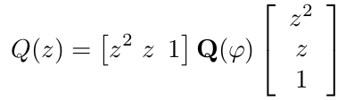
Here, the symmetric 3x3 matrix Q(φ) is as follows:
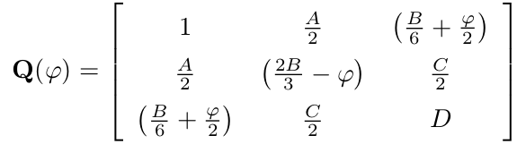
A symmetric 3x3 matrix has 6 independent parameters. All elements, which are not on the antidiagonal, are fixed by the coefficients of Q(z). For the antidiagonal, however, there is some freedom. The sum of these three elements must be equal to B, and the matrix must be symmetric. There is freedom in "distributing" portions of B over the antidiagonal, and there is the parameter φ, which can be chosen freely.
If the matrix Q(φ) is singular, then its rank is at most equal to 2 and in that case, it can easily be decomposed into a diagonal 2x2 matrix and two matrices, who are each other's transpose.
The matrix is singular, when det(Q(φ)) = 0. The determinant is a third-degree polynomial in φ. With the shown "distribution" of B over the antidiagonal (⅙ part on both corner elements and ⅔ part on the centre element), the third-degree polynomial in φ is a depressed third-degree polynomial of the form φ3 + gφ + h, where g and h depend on A, B, C, and D. Strobach discovered a property of the expressions for g and h, which allows one to compute these with high accuracy, even when they have very small magnitude, while the coefficients A, B, C, and D do not have a small magnitude. For any depressed third degree equation, it always is possible to at least compute one of the roots without numerical cancellation. Strobach calls this the dominant root. It also is easy to determine, which of its roots is the dominant one. This dominant root is called φ0.
So, Q(φ0) is singular and has rank at most equal to 2. The matrix can be decomposed as follows:
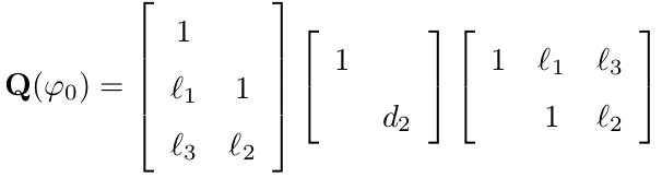
This is the so-called LDLT decomposition of the matrix Q(φ0). This decomposition can easily be determined for a small matrix like Q(φ0). The magnitude of d2 can be distributed over the matrix at the left and the matrix at the right as follows:

Here γ = √|d2|, and σ is the sign of d2 (-1 if it is negative, 1 if it is non-negative).
The quartic expression now can be written as

When all matrices are multiplied and the expression is written as a scalar, then a simple expression is formed, which can easily be factorized, using only quadratics.

where
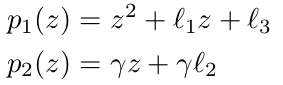
The quartic now can be considered solved. Either two real quadratic equations are obtained (if σ equals -1), or two complex quadratic equations are obtained (if σ equals 1). Each equation gives two roots of the quartic.
This algorithm is fairly simple. Its best property, however, is that analysis of all steps is much more feasible than is the case for Ferrari's solutions and other similar solutions methods. Strobach did an excellent job in analysing the possible sources of strong cancellation in the determination and solving of the depressed resolvent cubic equation, but in the accurate determination of l1, l2 and l3 he missed a few serious issues. These issues are beyond the scope of this web page, but they are described in the paper, given at the start of this web page.
![]()
The algorithm, described in the paper, and implemented in Java and C, is really robust and it also is quite fast. It is nearly as fast as a purely analytical solver, and its accuracy is close to what is theoretically attainable. Only in very few situations (one out of tens of millions of randomly generated equations) the accuracy is one digit less than what can be attained theoretically. The solver also achieves theoretically attainable accuracy when there are multiple roots, or closely clustered roots.
Up to now, I could not find any quartic equation, which could not be solved satisfactorily by the solver. If someone finds such an equation, then I really would like to know of it. I already used the solver in many mathematical experiments and solved billions upon billions of equations with it and did not find any issue with them. Using the provided test software, I also tested well over 1011 equations, all of them having good accuracy.