

Sine wave oscillator driven into chaos
This is an experiment, demonstrating how a simple sine wave oscillator can be driven into chaos, which very much resembles the chaos, exhibited by the classical Rössler dynamical system.
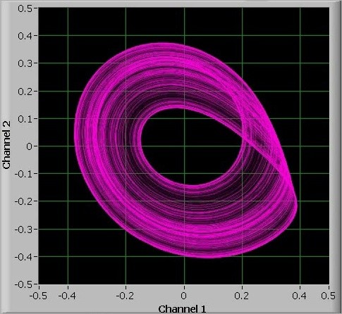
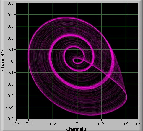
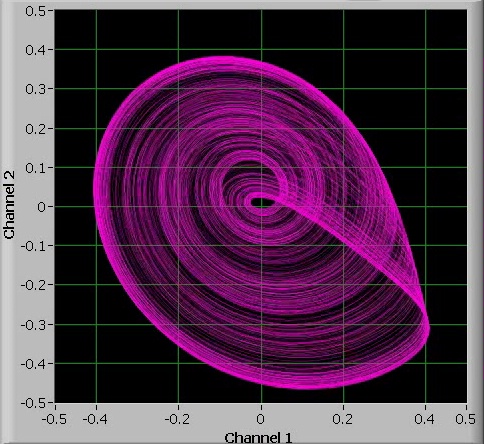
A simple electronic circuit was built which exhibits Rössler-like chaotic oscillation. Two output signals were displayed on an oscilloscope in X-Y mode. The picture below shows the output signals of this circuit for a certain choice of components. This very much resembles the appearance of the chaotic attractor of the Rössler dynamical system, projected on the x-y plane.
In this webpage the mathematics of the harmonic oscillator is taken as a basis. A connection is made with the classical Rössler oscillator and from a qualitative analysis of the behavior of the Rössler model, a new set of equations is derived, which easily can be approximated in a real electronic circuit costing no more than $3 and using only standard components which can be purchased without problem in any electronics store.
The Rössler oscillator
In 1976 the German biochemist Otto Rössler found a set of three differential equations, which shows interesting chaotic behavior for certain choices of parameters. The system he investigated is remarkably simple and it can be described by three differential equations with just one non-linearity:
![]()
![]()
![]()
Here, xr, yr and zr are the state variables of the system and a, b and c are constant parameters. The system only contains one non-linearity and that is in the equation for zr, where there is a product zr∙xr. Otto Rössler was interested in this particular set of equations because he used it to model the kinetics of a certain type of chemical reaction, but later on the study of the dynamics of this system has become a science on its own, due to its remarkable simplicity, yet being capable of intricate and really interesting behavior.
In this web page the Rössler system is viewed from a rather different point of view and a whole class of dynamic systems can be constructed which exhibits exactly the same type of chaos as the original Rössler system. In order to do so first some basics of the harmonic oscillator are explained.
The harmonic oscillator
Any physical system with two degrees of freedom, which can be described by the following differential equation can be regarded as a harmonic oscillator:
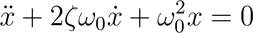
The solution of this second order differential equation is a sinusoidal signal x(t), with amplitude and phase depending on the initial conditions x(0) and x'(0). The equation for the harmonic oscillator contains two parameters, ζ and ω0. The parameter ζ is called the damping ratio and ω0 is called the undamped angular frequency. The general solution of this equation can be written as
![]()
When the damping ratio equals 0, then the output signal x(t) is a purely sinusoidal signal, which can be written as
![]() ,
,
where A and θ depend on the initial conditions x(0) and x'(0).
When the damping ratio is positive, then for any initial conditions the oscillation amplitude goes to 0 asymptotically. When the damping ratio is negative, then the oscillation amplitude grows exponentially without limit.
Constructing a harmonic oscillator (or good approximations) can be done in many physical domains. A few examples of harmonic oscillators:
- Mass-spring system, where the position of the mass, relative to the position at rest, takes the role of the variable x(t).
- Capacitor-inductor circuit with the two terminals of the capacitor connected to the two terminals of the inductor. In this system the voltage across the capacitor takes the role of the variable x(t).
- Pendulum swinging at low amplitude in a constant gravitational field (for larger amplitude the non-linear behavior of this system becomes more and more apparent). The swing-angle takes the role of the variable x(t).
All realizations of the above examples of harmonic oscillators have a positive damping ratio, due to friction or electrical resistance. In order to keep the oscillator going, an external energy source is needed, which compensates for the loss of energy due to friction or resistance.
In mechanics there is a system called escapement, which can be used to convert a constant torque into a timed 'kick' of a pendulum. The torque is supplied by a mass on a chain, or by winding a spring in a watch.
In electrical systems, active components like transistors or opamps combined with a suitable power supply are used as an energy source for keeping the oscillation going. An electrical equivalent of the harmonic oscillator is presented below and it is derived how this can be constructed easily, using just a few opamps, two capacitors and a few resistors.
![]()
Relation of harmonic oscillator with Rössler system
The harmonic oscillator's second order differential equation can be rewritten as a set of two first order differential equations in which the undamped angular frequency is a design parameter and the damping ratio is another design parameter.
Introduce a new variable y such that
![]()
Using this, one can write
![]()
The differential equation for the harmonic oscillator then can be written as
![]()
Rearranging terms and dividing by ω0 gives the following two combined equations:
![]()
![]()
These equations can be scaled by means of a simple transformation, such that ω0 disappears from the equations. Using a time scaling, where time is running ω0 as fast as real time, we can rewrite these equations in the form
![]()
![]()
Here xs and ys are the time-scaled versions of x and y. In these scaled equations, the dot stands for the derivative with respect to scaled time ω0t.
If these equations are compared with the Rössler equations, then there is a striking resemblance with the first two equations of the Rössler system. When the Rössler parameter a is taken equal to –2ζ then the only remaining difference is the insertion of the term zr in the time derivative of xr. So, the Rössler system can be regarded as a harmonic oscillator with damping ratio equal to –a/2 and some additional non-linear term.
![]()
![]()
The black part of the Rössler equations can be regarded as a harmonic oscillator and the red part as a non-linear perturbation.
Kick back mechanism in Rössler-like systems
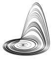
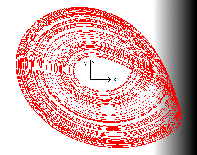
If one looks at the behavior of the Rössler system, then for positive a it can be regarded as a harmonic oscillator with negative damping ratio, resulting in oscillation with ever increasing amplitude. The state (x,y) spirals around the origin (0,0) outwards. The term z can be regarded as a corrective 'kick' back whenever the amplitude of x becomes too large. This 'kick' does its work while y is near 0, so effectively the system is brought back to a situation, where its state is closer to the origin. The 'kick' is not hard, but its strength sharply increases when x goes beyond a certain invisible boundary at the right.
When the state (x,y) is in the white area of the figure below, then only the black part of the differential equations plays a role and for positive parameter a there is outward spiraling motion of (x,y), but the more x goes to the right, the more the corrective term z play a role. In the figure below this is demonstrated by the grey/black band. The longer the state variable x remains in the gray area or the deeper the x value goes into the grey area (darker grey), the stronger the 'kick' back towards 0 some time later.
It appears that the precise nature of the 'kick' is not important, as long as the kick does not do its work immediately when x goes through some invisible boundary at the right. If the state variable x is pushed backwards immediately when it goes beyond a certain boundary at the right, then its action simply is to stabilize the oscillation and the system oscillates producing a somewhat distorted sine wave signal. When the state variable x is allowed to grow further for some time before the 'kick' sets in, then different kinds of interesting behavior can be achieved, including period doubling and chaos. Delayed kick back can only be achieved by adding another dynamic element to the system, hence increasing the order of the system from 2 to 3. This is in agreement with theory of nonlinear dynamic system, which states that the order of a time-continuous dynamic system must be at least equal to 3 for exhibiting chaotic behavior. Second order dynamic systems are capable of demonstrating oscillatory behavior, but not chaotic behavior.
In the Rössler system, the delayed 'kick' back is achieved by means of the following equation:
![]()
This equation is written in red, because it is part of the 'kick' back subsystem and not part of the basic harmonic oscillator. When this subsystem is studied in more detail, then it can be regarded as a simple first order system in zr with negative feedback when xr is low and positive feedback when xr becomes large. In the Rössler system, the parameter b is chosen small and its precise value does not really matter. A suitable value is 0.2, but 0.3 is equally suitable. In many studies of the Rössler system, the value c is taken somewhere around 5. As long as the state variable xr remains below 5, zr remains small and its effect on the harmonic oscillator is small, but as soon as xr goes beyond 5, there is positive feedback for zr and it grows exponentially in time. When xr goes deeper into the grey/black area of the figure above, then the positive feedback for zr becomes even stronger and zr grows at an amazingly high rate. So, if xr stays in the grey area for a somewhat longer time or it penetrates into the area deeply, then the kick back is strong. If xr just touches the grey region, then there only is a gentle push backwards.
The following graph demonstrates the kick back mechanism for a Rössler-like system. When x reaches a large positive amplitude and goes into the grey region, then z rapidly grows and this results in a sharp backwards kick of x and one can see a sharp non-linear change of x when z is large. With the fall of x, the value of z also quickly falls back towards 0 again.
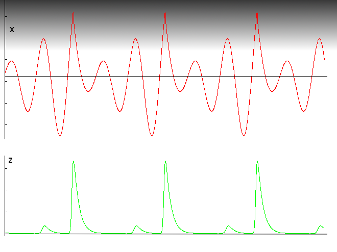
Any mechanism, which provides a delayed kick back when x exceeds a certain value can lead to qualitatively similar behavior. The exact shape of the z-spike is not important, only the qualitative effect is needed to achieve the kick back.
![]()
Experiments with an electronic realization of a Rössler-like system
All the above is a nice piece of theory, but it is even better to see how things work in a real system. So, the task is to find a method of generating a delayed kick back, which kicks in when the amplitude of a certain signal x becomes large, and combine this with a harmonic oscillator with adjustable negative damping ratio.
Nonlinearity for generating high spikes for sufficiently large x
The original Rössler system uses a non-linearity of the form z∙(x–c), which introduces negative feedback for small x and positive feedback for large x, introducing exponential (and hence very fast) growth of z for large x. Although a nonlinearity of the form z∙(x–c) can be created in electronics fairly easily, using a transconductance amplifier (such as the CA3080 or LM13700) or an analogue multiplier (such as the AD633), an even simpler method of generating a qualitatively similar spike-generating nonlinearity exists, using just a simple diode and normal opamps.
Mathematically the nonlinearity in the circuit looks totally different, but the qualitative behavior is similar to the behavior of the nonlinearity in the original Rössler system.
In this experiment the following nonlinear circuit is used:
In this webpage, more background information is given and it is explained why this circuit provides the desired behavior.
The harmonic oscillator
The other part of the circuit must be a linear harmonic oscillator, in which the value of z can be injected easily. A well-known type of linear harmonic oscillator, which gives both sine and cosine waves is the so-called quadrature oscillator. The quadrature oscillator is an oscillator, which produces both a sine and a cosine wave and it is based on the formation of a loop of two integrators. With opamps, it is really easy to make a pure integrator, having both polarities of the output available (positive and negative of integral). With modern dual-opamp integrated circuits, only one small 8-DIP package is needed:
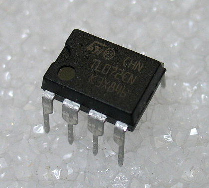
This 8-DIP package is used in conjunction with three resistors and one capacitor for building a complete integrator:
This circuit also easily can be extended, such that other signals are added to the input. For each additional signal, which also needs to be integrated, one only needs to add a resistor R and connect that to the inverting input of the left opamp. In such a configuration one easily can integrate sums of signals.
With these building blocks available it now is easy to derive the complete circuit for the chaotic oscillator. In the diagram all three sections for x, y and z are drawn. In order to complete the circuit, the outputs x, y and z (or the negatives of them) must be connected to the inputs at the left.
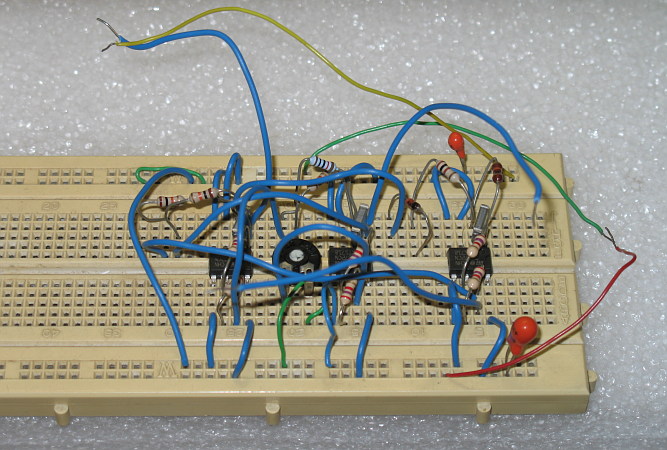
This circuit shows chaotic oscillating behavior for a very wide range of RC combinations. Nice results with oscillations around 1.5 kHz are obtained when R is taken equal to 10 kΩ and C is taken equal to 10 nF. Three dual opamp IC's are needed, and the type of this circuit is not critical at all. This experiment was conducted with humble low-cost TL072 dual opamps, but any opamp, internally compensated for unity gain, will do the job. The DC characteristics of the opamps do not matter at all. Tests were done with artificially created offset voltages as high as 100 mV and no ill effects on the capabilities of the circuit were detected. The circuit is robust and always starts oscillating, when switched on. Output amplitude of the signals is in the order of magnitude of 0.4 volts. The resistor R/a can be implemented by using a series connection of a fixed resistor of 22 kΩ, connected in series with a 250 kΩ potmeter. This allows values for a to be adjusted between 10/272 and 10/22, which is 0.037 to 0.45. Over this range, a lot of interesting behavior can be achieved. A breadboard "chaotic circuit" was built and this was used for experimenting.
When the potmeter is turned from low value of a (highest resistance) to high value of a (lowest resistance), then a truly amazing series of events occur. The system starts like a normal quadrature oscillator, producing a sine wave and a cosine wave. When an X-Y plot is made on an oscilloscope, the result is a simple slightly distorted circle:
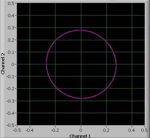
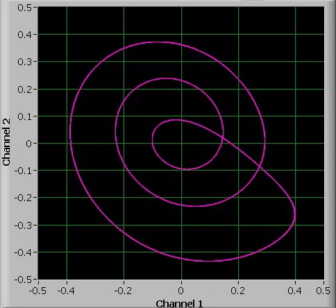
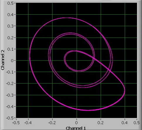
When the value of a is increased, then the circle deforms and at a certain point, a so-called period doubling (bifurcation) occurs. Now the system needs two cycles, before the same situation is reached again.
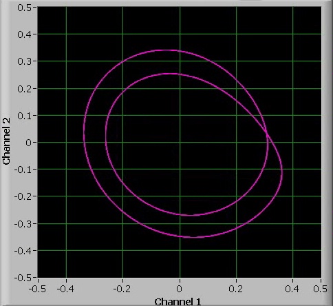
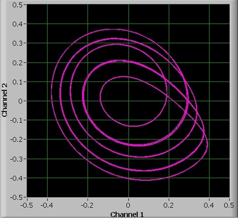
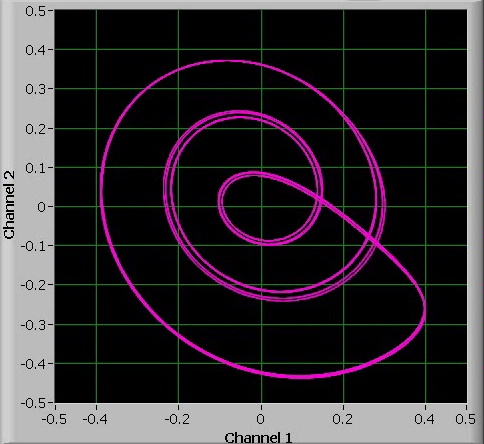
When the value of a is increased further, then other bifurcations occur. The bifurcations follow each other more and more quickly when turning up the value of a. The width of the interval from one bifurcation to the next bifurcation decreases exponentially. The next two pictures show a 4-period bifurcation and an 8-period bifurcation.
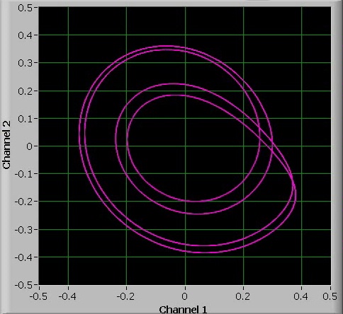
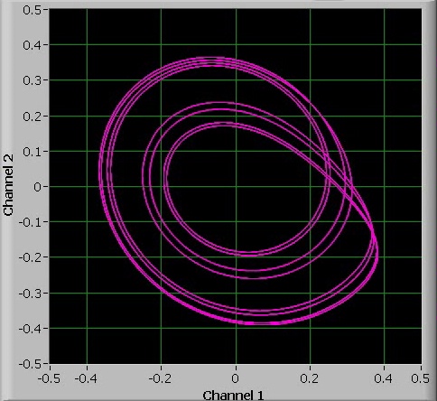
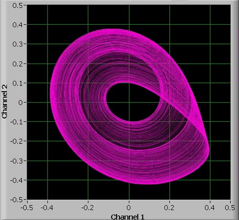
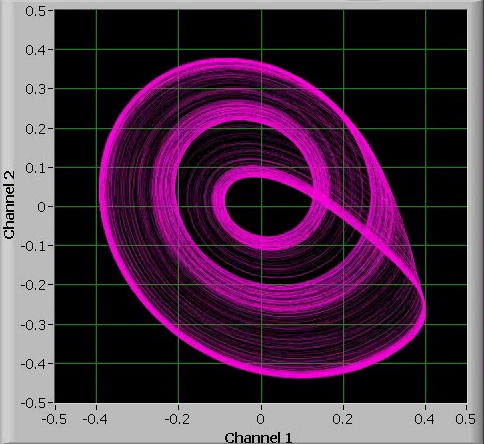
More than period-8 oscillations can hardly be observed. Turning up the value of a slightly above the period-8 oscillation, as shown in the last picture above, results in chaotic behavior.
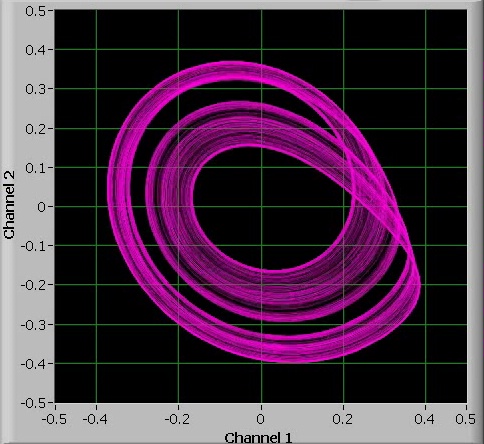
When the value of a is increased further, then the chaos becomes less banded and the amplitude of the oscillations varies wildly:
At a certain point, however, suddenly a periodic oscillation appears again. This time, a 5-period oscillation can be observed.
The interval in which there is such a 5-period oscillation is very narrow and it is hard to keep this oscillation really stable. It seems to jitter somewhat between 5-period and 10-period oscillation (a bifurcation).
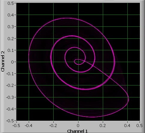
When the value of a is further increased, then chaos sets in again, but at a certain point, there suddenly is a 3-period oscillation. This 3-period oscillation appears over a fairly large interval of a. It also is possible to observe the 6-period bifurcation and 12-period bifurcation of this 3-period cycle.
Again, increasing the value of a even more leads to chaos again:
But at a certain point, there is a 4-period oscillation. This 4-period oscillation is of a different nature than the 4-period oscillation, which stems from 2 bifurcations of the single-period oscillation. The oscillation, observed here is an exponentially increasing signal for 4 periods and then a single strong kick-back, while the 4-period oscillation, which stems from the single-period oscillation is a situation, where there is a mild kick-back in each cycle.
Again, also for this 4-period oscillation, there is onset to chaos when the value of a is increased further.
It is rather interesting to see how a small circuit with less than $3 of electronic components in it shows such rich chaotic behavior.
A video of the behavior of the oscillator was made, while the non-linear kick-back was turned up slowly from very weak to quite strong. The potmeter was turned from one side to the other side very slowly and in the meantime the video was made. Download size is appr. 7 MByte.
![]()
Simulation of diode-based chaotic oscillator
The same circuit also was simulated, using a small computer program written in Java. The Java program contains a general differential equation solver, using the well-known Runge-Kutta workhorse for solving differential equations. It might not be the most efficient method, but it is robust and easily programmed. The main-method uses this Runge-Kutta differential equation solver to step through the solution in steps. The source code can be downloaded here. Unpack the file (it contains an src-directory with three package directories in it) and compile this program using an IDE like Eclipse or Netbeans. When the program is run, then an output file is generated with the name "c:\rossler.txt". For the current parameter setting this output shows a three-period cycle.