Remarkable properties of roots of polynomials

This is a set of experiments, using advanced software for finding zeros of polynomials. First it is briefly explained what is meant with the word "polynomial". Next, the concept of polynomial equations is introduced, and finally, different types of polynomials are explored and some beautiful patterns of roots of polynomial equations are shown. An example is given in the picture below of the complex zeros of a 1000^th degree polynomial. The software, used for the experiments, described in this web page, is available in source code format and can be compiled for Linux, Windows, and ARM systems like the Raspberry PI or Odroid C1, and Odroid C2.

For people with somewhat more mathematical background, the first few paragraphs of this webpage may be dull and full of trivial contents, but the introduction to polynomials is added so that everyone with knowledge of upper level high school mathematics can understand what happens in this web page.

What is a polynomial?

The word "polynomial" is a strange word derived from two languages, which first appeared in the 17th century. It is a combination of the Greek word "poly" and the Latin word "nomen". This makes its literal translation "multiple names".

In mathematics, a polynomial is an expression, consisting of terms, where each term is a non-negative integer power of some variable or unknown, multiplied by a constant. A few examples of polynomials are given below:

• polynomial in one variable x : 5x² + 10x − √2
• polynomial in two variables x and y : −5x²y³ + x⁴ − π xy + 17
  

As the examples show, the constant factors may be anything, as long as they do not depend on the variables in which the polynomial is expressed.

This web page is about polynomials in a single variable. This kind of polynomial is called univariate polynomial.

A polynomial can be regarded as a mathematical function, which only contains integer powers of the argument of the function. The univariate example, given above can be written as

p(x) = 5x² + 10x − √2

The degree of a univariate polynomial is the highest power of the variable which appears in the expression. In this example, the highest power is 2, hence the degree of that polynomial is 2.

A general expression for an n^th degree univariate polynomial in variable x is

a₀ + a₁x + a₂x² + . . . + a_nxⁿ, where a₀, a₁, a₂, etc. are constants. These constants are called coefficients. Terms with coefficients equal to 0, usually are not written. E.g. 5 + x³ is a 3^th degree polynomial with coefficients a₀=5, a₁=0, a₂=0, a₃=1. The order in which terms appear in a polynomial does not matter. Sometimes people write polynomials with highest powers at the end, other times they write polynomials with highest power first. A 0^th degree polynomial is simply a constant.

Polynomials can be defined over any field. This webpage restricts itself to polynomials over the field of real numbers or the field of complex numbers. A polynomial over the field of real numbers has real coefficients, a polynomial over the field of complex numbers can have real coefficients, but it also may have complex coefficients.

Zeros of polynomials

A zero of a polynomial p(x) is a value x₀, which can be substituted for x, such that p(x₀) equals 0. Sometimes such a number also is called a root. For example, the roots of the equation x² − 5x + 6 = 0 are the numbers 2 and 3. These numbers are called the zeros of the polynomial x² − 5x + 6. A polynomial over the field of real numbers does not need to have any real zeros. E.g. the polynomial x² + 1 has no real zeros. There is no real x, which can make x² + 1 equal to 0. Finding real zeros of low degree polynomials with real coefficients can be done graphically, by drawing the graph of the function p(x).

A polynomial also can have a so-called multiple zero. This means that it has zeros of the same value. What is meant with multiple zero (in this case a double zero) is demonstrated by a simple graphical example.

Here you see  the graph of p(x) = x³ − 3x² + 4. This polynomial has two distinct zeros, one being equal to −1, the other being equal to 2. The zero at 2, however is a double zero. The graph passes through the x-axis at x=−1. At x=2 it just touches the x-axis. Imagine another polynomial q(x) with the graph of p(x) moved down a tiny amount ε: q(x) = p(x) − ε = x³ − 3x² + 4 − ε. You see that the double zero 2 splits up in two distinct zeros 2−δ₁ and 2+δ₂, where δ₁ and δ₂ are small amounts, depending on the precise value of ε (for very small ε, δ₁ ≈ δ₂ ∼ √ε). The zero at −1 also changes slightly, but it remains single. When the graph of p(x) is shifted upwards, then the double zero at 2 disappears and only a single zero near −1 remains. 

A full understanding of the roots of polynomial equations only is possible when one is working in the field of complex numbers. It goes too far to explain complex numbers in this webpage. A good introduction to complex numbers can be found on internet, e.g. https://en.wikipedia.org/wiki/Complex_number.

In the field of complex numbers the above example can be understood better. When the graph is shifted upwards a tiny amount ε the double zero at 2 splits into two distinct complex zeros, which for very small ε can be approximated well as 2−δi and 2+δi, with δ ∼ √ε. So, in the field of complex numbers, the total number of zeros is equal to 3, regardless of how much the graph is shifted. We either have 3 distinct real zeros, one real zero and one real double zero, or one real zero and two complex zeros. The total number of zeros, however, always equals 3. The situation with the double zero is a borderline situation. Distinct zeros have a so-called multiplicity. A normal (single) zero has multiplicity 1, a double zero has multiplicity 2, a triple zero has multiplicity 3, and so on.

Fundamental theorem of algebra

In the field of complex numbers, in general a polynomial of degree n has at most n distinct zeros, but if the multiplicity of zeros is taken into account, then a polynomial of degree n has exactly n zeros. This is a very important theorem, and it is called the fundamental theorem of algebra. Keep in mind though that this only is true in the field of complex numbers. In the field of real numbers, the number of zeros may be less than the degree of the polynomial and in other fields the number of zeros also may be less.

Any polynomial over the complex numbers can be written in product-form if its zeros x₁, x₂, . . ., x_n are known.

p(x) = a₀ + a₁x + a₂x² + . . . + a_nxⁿ = a_n (x−x₁)(x−x₂) . . . (x−x_n)

Some of the zeros may have the same value, in that case we have a multiple zero. The example polynomial x³ − 3x² + 4 can be written as (x+1)(x−2)(x−2).

Finding the zeros of polynomial equations

The fundamental theorem of algebra only states something about the existence of zeros, it does not tell anything on how to find the roots of polynomial equations. For first degree and second degree polynomials, finding the zeros is easy. This is thought at high school. It also is possible to provide expressions for the roots of 3^th degree and 4^th degree polynomial equations, in terms of √, ∛, ∜ and the arithmetic operations +, −, ∙, and /. For higher degree polynomials no general formula in terms of n^th-roots and basic arithmetic operations exists. It is not a matter of not yet having discovered such a formula for e.g. 5^th degree polynomials, but it is proven that no such formula can exist for general polynomials of 5^th or higher degree. Understanding that kind of proof is beyond high-school mathematics and only a reference is given here: https://en.wikipedia.org/wiki/Abel%E2%80%93Ruffini_theorem.

Just for fun, the formula for second degree and third degree polynomials is given here for comparison. The formula for one of the zeros of a general fourth degree polynomials is insanely complicated and would fill many pages.

The zeros of the second degree polynomial ax² + bx + c can be written as

One of the zeros of the third degree polynomial ax³ + bx² + cx + d can be written as

The formula for the third degree equation only gives one zero, the one which always is real for real coefficients a, b, c, and d. For the other two zeros there are similar but somewhat more complicated expressions. If the third degree equation has three real roots, then the above formula has a real value, but the two cube root terms are complex. The imaginary parts of these terms cancel exactly. A nice page, which also gives a good derivation of the expressions for roots of third degree polynomial equations, can be found on Wikipedia: https://en.wikipedia.org/wiki/Cubic_function.

Numerical approximation of zeros of polynomials

As stated above, there is no general applicable formula, which gives the roots of any given n^th-degree polynomial equation. It, however, is possible to find numerical approximations of the zeros of polynomials. For low degree polynomials with real coefficients, one can draw a graph and find estimates of the real roots. This is nice for high school mathematics and can be done on modern graphical calculators, but for general unattended root-finding this method is not very useful.

In the last decades a lot of research-effort is put in finding reliable methods for approximating roots of general polynomial equations. This has proven to be a remarkably difficult task. Nearly all algorithms, developed over the last 100 years, work for many polynomials, while they fail miserably for many other polynomials. Only recently, really fool-proof algorithms became available. A really amazing algorithm is the 2012 incarnation of the MPSolve algorithm by Dario A. Bini and Leonardo Robol. Also from Bini, there is a Fortran implementation of 1996 of a limited precision implementation of a much older version of the MPSolve algorithm. There also are much-praised algorithms from M.A. Jenkins and J.F. Traub, implemented in Fortran around 1970. Some of these algorithms I ported to C and to Java and for the 2012 MPSolve algorithm I developed a so-called JNI interface so that my implementation in C becomes available from Java-programs on PC's running under Windows or Linux. There also is a JNI implementation for 32-bit and 64-bit ARM architectures (e.g. Raspberry PI, Odroid, Orange PI). The source code and instructions for how to compile and run these programs are given in a separate page: software.html. Bini and Robol themselves also provide an implementation of their 2012 MPSolve algorithm, but this implementation has many bugs (a lot of memory leaks and a completely borked piece of code for estimating the accuracy of the results obtained so far). This not so good implementation, however, also makes clear how robust their mathematical algorithm is. Even with a buggy implementation, which sometimes completely screws up computed intermediate approximations, the algorithm still gives good results, albeit at higher computational cost. I created an implementation, loosely based on Bini's and Robol's code, but it is (as far as I know) free of memory leaks and much faster for high precision output calculations.

The 1996 MPSolve algorithm and the Jenkins and Traub algorithm use standard floating point arithmetic with double precision of 53 bits, or a double double precision of 105 bits, which is made available for both C and Java through a fairly simple set of functions/methods. The 2012 MPSolve implementation uses GMP, a multi-precision library, and allows computations at very high precision (thousands of bits is not uncommon) at the cost of higher computation time. The code, using 53-bit or 105-bit precision can be used to solve polynomial equations of degree up to 50 or so, having not too difficult configurations of roots (e.g. tight clusters of roots, or multiple roots). A single double root or even triple root, well separated from the other roots, however, can be handled by that code.

The implementation of the 2012 MPSolve algorithm can be used to find zeros of polynomials of degrees 10000 or even higher if you are patient. This software has no problem with tight clusters of roots, many multiple roots and other extremely ill-conditioned problems. Up to now, I could not find a single polynomial equation, which could not be solved by the 2012 MPSolve implementation! This program is very interesting for exploring extremely high degree polynomials.

The algorithms behind the software are beyond the scope of this webpage, but in the software itself, there is extensive documentation and there also are copies of relevant papers. This webpage from now on emphasizes on exploring some interesting classes of polynomial equations.

Exploration of truncated power series of exponential functions

The exponentional function f(x) = e^x has no zeros. The Taylor series of this function is as follows:

This series has no zeros, but what if the series is truncated? We can obtain a polynomial of n^th degree by truncating this series after the term with power n. The truncated power series can be written as

According to the fundamental theorem of algebra, this truncated series has exactly n solutions in the complex plane. For n going to infinity, the number of zeros of the truncated power series equals n. Here we seem to have a paradox, because f(x), which is f_∞(x) has no zeros, while we expect it to have ∞ zeros. This interesting seemingly paradoxical situation can be investigated by approximating the solutions of f_n(x) for increasing values of n. Below follows an animated GIF image of the zeros of the truncated power series of f_n(x) for n ranging from 10 to 1000. As the animation shows, for increasing n, the magnitude of the zeros increases.

What if n goes to infinity? Because of the fact that f(x), the infinite series, has no zeros, one could conclude that the zeros go to infinity as well. Another test is done to confirm this. I also made an animation, for which the zeros of f_n(x) were approximated and then these zeros, divided by n, were plotted in the image. So, the zeros are scaled down with the value of n, for which the power series is truncated. A link to this animation is given here: zeros of f_n(x), divided by n. This animation shows that the zeros, divided by n, seem to converge to points on a certain curve. This is strong evidence for the hypothesis that the roots of the truncated power series f_n(x) go to infinity if n goes to infinity. The exponential function hence has an infinite number of zeros at infinity!

The fact that the scaled zeros of the truncated power series f_n(x) converge to points on a certain curve is a very deep result. Even deeper is that an analytic expression is found for this curve. This great result is obtained in the 1920s by a hungarian mathematician, called Gábor Szegö. The zeros of the function f_n(nx) converge to the curve ∣ze^z−1∣ = 1, where z is a complex number. In this paper a thorough derivation is given of this result. This curve nowadays is known as the Szegö-curve.

All zeros near the Szegö-curve are an artifact of the fact that the power series is truncated. As n is increasing, the curve blows up (unscaled). This matches with the fact that the equation e^x = 0 has no zeros. Next comes a very interesting observation, about general equations e^x − p(x) = 0, with p any polynomial of x.

Generalized exponential equations of the form e^x − p(x) = 0

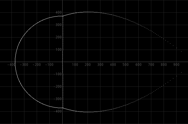
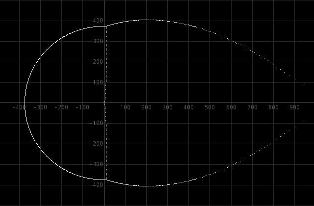
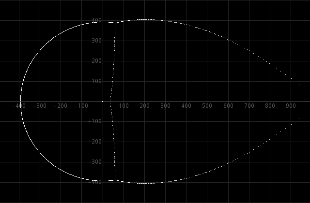
No analytical expressions can be given for the solutions of the generalized equation e^x − p(x) = 0, with p a polynomial of x. For constant (0^th degree) polynomials a₀, this equation can be solved. There are infinitely many solutions in the complex plane, which can be written as ln(a₀) + 2kπi for any integer value of k. What happens with the zeros of the truncated power series of e^x − a₀? Below, the solutions are shown for a constant polynomial p(x) = a₀ = 1.

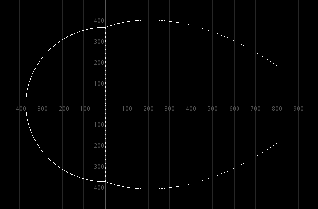
This image shows zeros at the imaginary axis, until the Szegö-curve is reached. At the left, the zeros are on a near-perfect half-circle, on the right, the zeros are near the Szegö-curve. When the numerical values of the zeros on the imaginary axis are inspected, then you see that up to many decimal places these zeros are close to 2kπi, the true zeros of the equation e^x − 1 = 0.

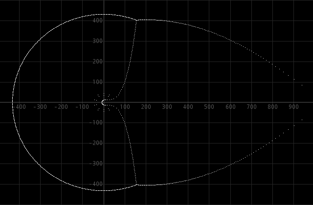
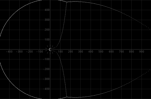
When we do a similar computation for e^x − x = 0, e^x − x² = 0, and e^x − x¹⁰ = 0, then we get very similar results:

Further analysis shows that the roots near the imaginary axis are very close to the true roots of the equations e^x − x = 0, e^x − x² = 0, and e^x − x¹⁰ = 0.

Similar results also are obtained for equations like e^x − 5x = 0, e^x − ½x² = 0, and e^x + x¹⁰ = 0.

Also, when more complicated polynomials are used, the results are similar. The following shows the result for the truncated power series of e^x − x³⁰_/30! − x⁴⁰_/40!  − x⁵⁰_/50! = 0. All zeros inside the outer curve are very good approximations of the true zeros of the untruncated function.

Finally, the effect of truncating at a larger power is shown. When the exponential function is truncated after the 1200^th term, then one sees that the roots in the interior of the combined circle/Szegö curve are not affected, but the circle/Szegö curve is blown up and additional very good approximations of true roots of the equation are added to the set inside the circle/Szegö curve.

This behavior, as demonstrated above, allows us to approximate true zeros of equations of the form e^x − p(x) = 0 simply by solving a truncated version for a certain n, such as n=1000, and solving a truncated version for a larger n (e.g. 10% larger). Roots, which are present in both sets (within an accuracy of 10 digits or so), are good approximations to true roots of this exponential equation, while the other roots are artifacts, due to the truncation of the power series of e^x.

All images, shown above, were generated with the help of a C-implementation of the 2012 version of the MPSolve algorithm, using GMP for the required high precision calculations. Solving one polynomial equation of 1000^th degree took approximately 30 seconds on an Intel Core i5, running at 3.4 GHz, in 4 threads, using all 4 cores simultaneously.

A complicated exponential equation

It turns out that similar behavior is obtained for more complicated exponential equations as well. In this experiment, a complicated equation is solved numerically and the obtained patterns are interesting. At the top of this webpage, the roots are shown of a truncated power series of the function

This complicated function can be written as a power series with complex coefficients. When this power series is trucated and the zeros of the resulting polynomials are determined, then the zeros at the interior are approximations of true zeros of this function, while the zeros on the outside are artifacts due to truncation of the power series. An in-depth study of this kind of sums of exponentials is given in this paper.

Using truncated power series of sine and cosine functions, one also can solve equations like sin(x) − x = 0 and cos(x) − x = 0. The functions sin(x) and cos(x) in fact are sums of exponential functions:

It is up to the reader of this page to experiment with this kind of functions. One can solve all kinds of combinations of sines and cosines and one can combine them with polynomials. In the accompanying software suite, you can find some Java-code which can be used to experiment with the sine and cosine truncated power series.

Effect of random perturbations on zeros of polynomial

A completely different method for exploring polynomial equations is to investigate how zeros move through the complex plane when the coefficients of the polynomial are perturbed. In this experiment the starting point is a chosen set of zeros of a polynomial and from this, all coefficients are determined, using a computer program:

   g(x)  =  (x − x₁)(x − x₂)(x − x₃) . . . (x − x_n)  =

                                     a₀ + a₁ x + a₂ x² + . . . + a_n−1 xⁿ⁻¹ + xⁿ

Next, the coefficients are perturbed, and a perturbed polynomial is determined:

  ĝ(x)  =  a₀(1+ε₀) + a₁(1+ε₁) x + a₂(1+ε₂) x² + . . . + a_n−1(1+ε_n−1) xⁿ⁻¹ + (1+ε_n)xⁿ

The perturbations are relative. If the perturbation ε_i equals 0.0001, then the coefficient a_i is perturbed after approximately the 4th digit. For many polynomials, such a small perturbation also leads to perturbations of the zeros in the same order of magnitude. For some polynomials, however, small perturbations of the coefficients lead to dramatic changes of the zeros.

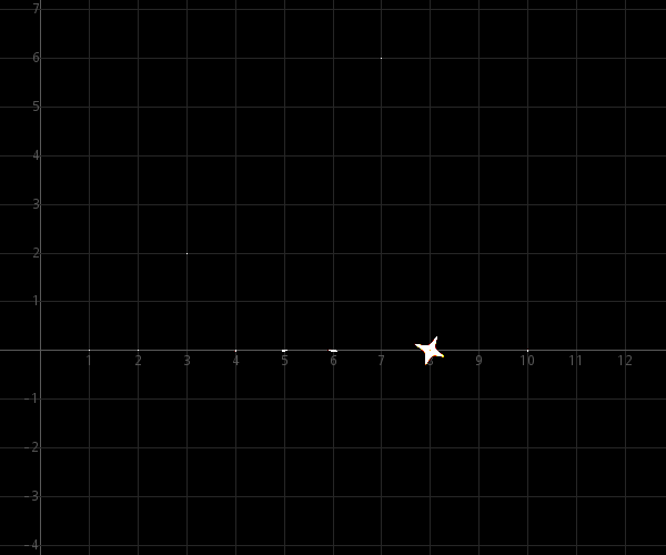
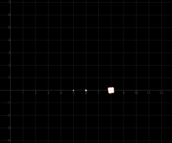
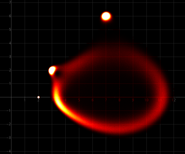
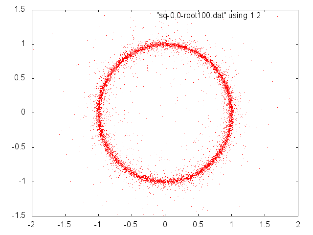
The polynomial (x-1)(x-2)(x-3-2i)(x-4)(x-5)(x-6)(x-7-6i)(x-8)²(x-10), which has complex coefficients, is used as a basis for the figures, shown below. The figures below are generated by first computing coefficients a₀, a₁, . . ., a₉. The coefficients a₁₀ equals 1. Starting from this polynomial, 2000000 random perturbed polynomials are created with ε₀, ε₁, ε₂, . . . ε₉, ε₁₀, randomly chosen from an interval [-ε_max, ε_max]. The zeros of each of these polynomials are computed and each zero is used to increase the "heat" of a pixel in an image. Each time a pixel is touched by a zero, it is made a little "hotter". When the image is rendered, then pixels, which are never touched are cold and black. Very hot pixels are white. Intermediate pixels are shades of red, orange, yellow at increasing "temperature". This kind of images nicely shows which areas of the complex plane are hit frequently, and which areas are never hit.

Multiple images are generated for multiple values of ε_max:

 ε_max = ½·10⁻⁷ :

 ε_max = ½·10⁻⁶ :

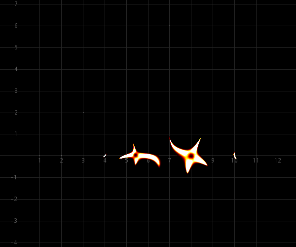
 ε_max = ½·10⁻⁵ :

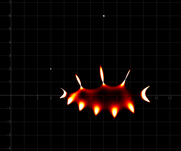
 ε_max = ½·10⁻⁴ :

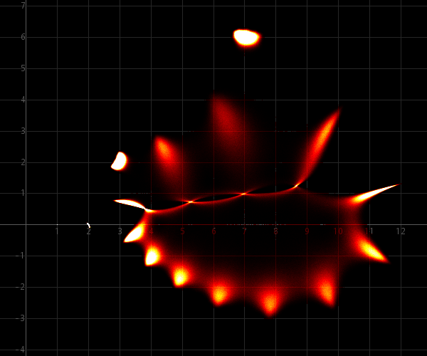
 ε_max = ½·10⁻³ :

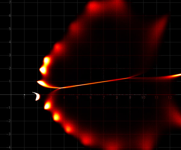
These images show intriguing patterns. The polynomial, used for this experiment, is nothing special, except that it has a double zero and that most of the zeros are on a line. This combination makes the polynomial very sensitive to perturbations.

An even more impressive demonstration of the behavior of the zeros of the polynomial under perturbation is a video, made from 81 images with ε_max ranging from ½·10⁻⁷ to ½·10⁻³, where the exponent goes from −7 to −3 in steps of 0.05. This video can be downloaded here. In order to make this video, 1.62 billion 10^th-degree polynomial equations were solved. This took nearly 70 minutes on an Intel Core i5 processor, running at 3.4 GHz, in a single thread. For this purpose, a Java implementation of the 1996 version of the MPSolve algorithm was used in standard 53-bit IEEE floating point precision.

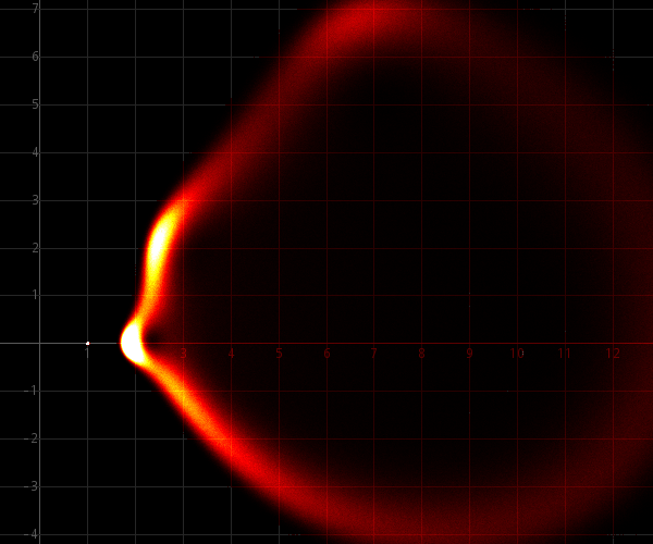
Separate random perturbations on real and imaginary part of coefficients

It is interesting to see the effect of using a slightly modified perturbation for the polynomial, given above. In the above situation, all perturbed coefficients â_i can be written as a_i(1+ε_i), where the relative perturbations ε_i are real numbers. The same experiment is done, where the real part and imaginary part of the coefficients a_i are perturbed independently. Suppose each coefficient can be written as

where μ_i and ν_i are random relative perturbations, computed independently from each other, both taken from a uniform random distribution in the interval [-ε_max, ε_max].
This only is a subtle change from the experiment, described above, where μ_i = ν_i.

Again, multiple images are generated for multiple values of ε_max:

 ε_max = ½·10⁻⁷ :

 ε_max = ½·10⁻⁶ :

 ε_max = ½·10⁻⁵ :

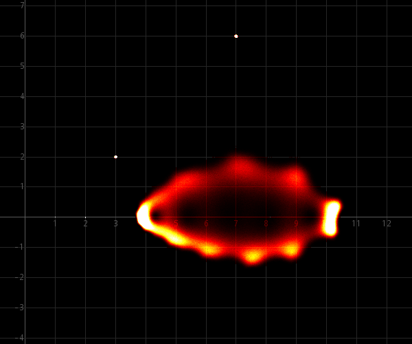
 ε_max = ½·10⁻⁴ :

 ε_max = ½·10⁻³ :

As these images demonstrate, the perturbed zeros are distributed more uniformly, but the difference is quite dramatic. This can be explained intuitively because for each coefficient, the perturbation space is a small 2-dimensional area, instead of a 1-dimensional part of a line. The effect will be a more fuzzy redistribution of roots.

Again, a video is made of this as well, again for 81 values of ε_max ranging from ½·10⁻⁷ to ½·10⁻³, where the exponent goes from −7 to −3 in steps of 0.05. This video can be downloaded here. The computation of this video also required solving 1.62 billion 10^th-degree polynomial equations and again, this takes nearly 70 minutes on an Intel Core i5, running at 3.4 GHz, in a single thread.

Random perturbations from disk with certain small radius

In this final set of experiments with random perturbations, the perturbations again are of the form a_i(1+ε_i), but now, the number ε_i is not a real number in a given interval [-ε_max, ε_max], but it is a random complex number in a disk of radius ε_max.  The complex relative perturbation ε_i is determined by picking a random number r_i uniformly from the interval [0, ½ε_max], and another random number ϕ_i picked from the interval [0, 2π>. The perturbation then is computed as

   ε_i = r_i e^{i ϕ_i} = r_i cos(ϕ_i) + i r_i cos(ϕ_i)

With this perturbation, the distribution of zeros looks quite different from the above.

Again, multiple images are generated for multiple values of ε_max:

 ε_max = ½·10⁻⁷ :

 ε_max = ½·10⁻⁶ :

 ε_max = ½·10⁻⁵ :

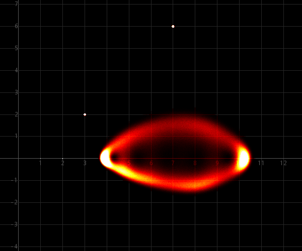
 ε_max = ½·10⁻⁴ :

 ε_max = ½·10⁻³ :

The perturbed zeros are distributed even more uniformly as in the previous experiment, but the difference is less dramatic.

Again, a video is made of this as well, again for 81 values of ε_max ranging from ½·10⁻⁷ to ½·10⁻³, where the exponent goes from −7 to −3 in steps of 0.05. This video can be downloaded here.

Distribution of roots of random polynomials

When a random polynomial is taken, with completely random polynomials, then for increasing degree of the polynomial, the roots tend to converge to the unit circle in the complex plane and their distribution on the unit circle tends to be uniform. This is true for many kinds of distributions, the requirements on the distribution are very weak. This also is true for many polynomials with non-random coefficients.

In fact, it is quite hard to find a polynomial of high degree which does not have roots near the unit circle. One really has to construct polynomials in order to find other distributions. Below follows a typical picture of the zeros of a polynomial of degree 300 with random coefficients, taken uniformly from the interval [27, 42]:

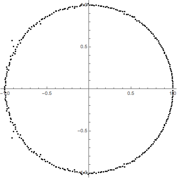
If a similar picture were made with coefficients, taken from e.g. [0, 100], [-10, 10], [30, 50] or even [-1000, 1000], then the result is very similar.

The following two figures show the effect of degree on the random roots. The higher the degree, the more the zeros approach the unit circle. The two figures below show zeros of several random polynomials of degree 10 and of degree 100, with coefficients taken at random uniformly from  the filled square [-1,1]+i[-1,1] in the complex plane.

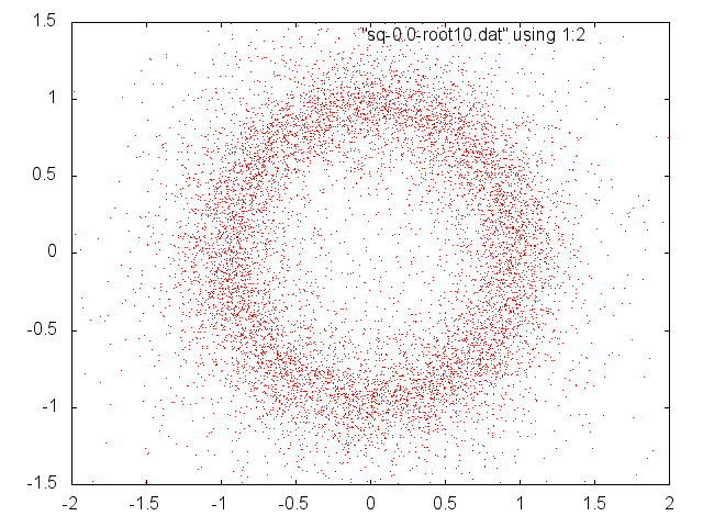
Inverse primorial polynomials

The section above shows that zeros tend to go to the unit circle for high degree polynomials. In this section, it is shown that other behavior can be constructed and quite interesting patterns emerge in this case. As a start, define the following analytic function on the complex plane:

Here, p_k stands for the k^th prime, and p_k# stands for the k^th prime primorial, which is defined as p₁·p₂ . . . ·p_k. It is the product of the first k primes. Some examples:

           p₁# = 2

           p₂# = 2 · 3 = 6

           p₃# = 2 · 3 · 5 = 30

           p₄# = 2 · 3 · 5 · 7 = 210

           . . . .

           p₈# = 2 · 3 · 5 · 7 · 11 · 13 · 17 · 19

The function ψ(x) is an analytic function on the entire complex plane. For people, who know of the concept of order and type of functions: it is an entire function of order ρ=1 and type σ=1/e². It grows exponentially fast for positive real x, at a rate comparable to e^x/e². For more info see https://en.wikipedia.org/wiki/Entire_function.

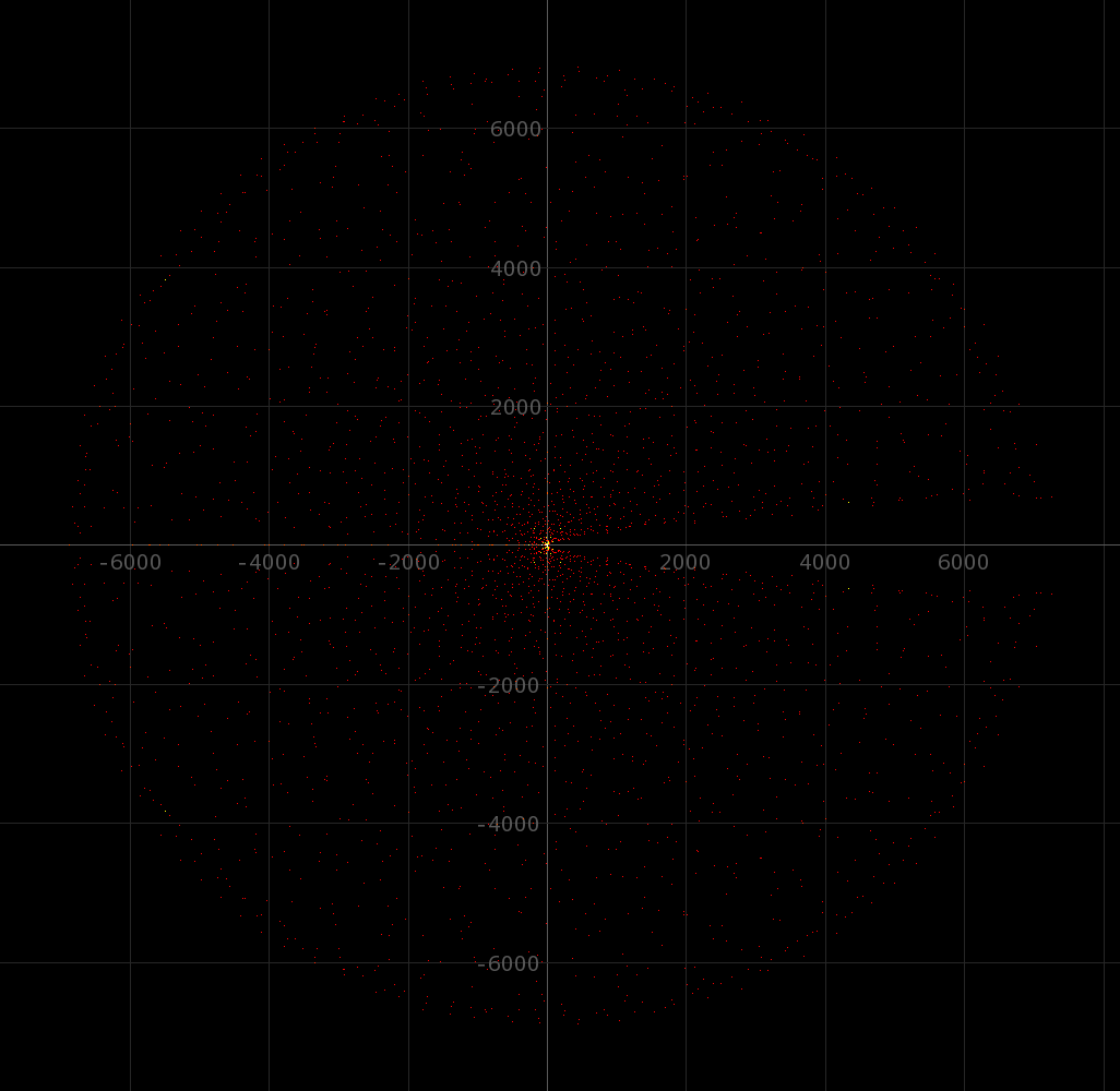
This function has infinitely many complex zeros distributed over the complex plane. Below, all zeros in the square from -10000 to 10000 in both real and imaginary direction are shown.

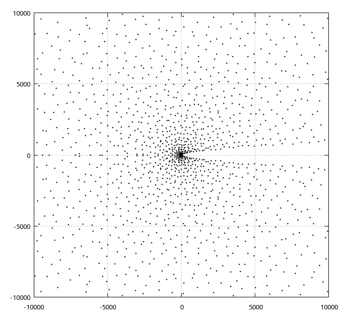
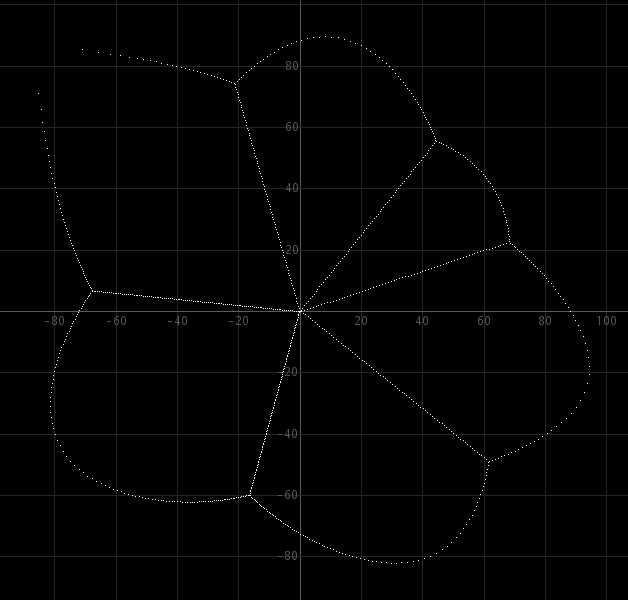
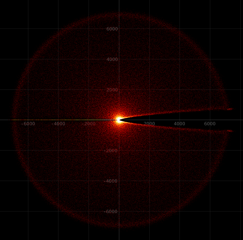
In the following image, all zeros in the square from -40000 to 40000 in both real and imaginary direction are shown.

These plots show that the zeros seem more or less randomly distributed, with density decreasing when the distance from the origin increases and there is an empty area around the positive real axis, which has no zeros at all. This is totally understandable. The function ψ(x) has positive coefficients for all terms in its power series, hence for any positive real number it has a positive real value and hence it has no zeros on the real axis. In order to get from the big positive real part to a point where the real part can become zero one has to move away from the real axis more and more for increasing values of x. This explains the widening band of no zeros around the real axis. The function has many negative real zeros in the range from −40000 to 0. The density of these also decreases with increasing distance from the origin. The graph of this function is a wildly and irregularly oscillating curve for negative real x, which occasionaly goes through the real axis.

The interesting thing is that approximating all these zeros from this analytical function can be done with the 2012 version of the MPSolve algorithm, by approximating zeros of different truncated power series. One series was truncated after power 7000 and the other after power 10000 and all zeros which are in both sets (within 12 digit accuracy) are genuine zeros.

A video demonstrates what happens when zeros of the truncated power series of ψ(x) are displayed, for polynomials of increasing degree. This video was created by rendering a plot of all the zeros of the n^th degree truncated power series in an image file. Such an image file was generated for each n in the range 2, 3, 4, . . ., 1600. All these image files were combined into an animated gif file.

A similar video was made, but now all zeros of the n^th degree truncated power series and all zeros of all lower degree truncated power series are accumulated into a single image and pixels are made hotter when they are touched more frequently. A pixel which is hit once is fairly dark red, a pixel which is hit several times becomes white hot. The genuine zeros will be hit many times for all truncated power series starting from a certain n. For each n in the range 2 . . . 1600 an image with all accumulated zeros is generated and these images again are put in an animated gif in order to obtain a playable video. This video shows intriguing patterns. There still is a lot to be investigated in the nature of these patterns.

It is best to watch these videos unscaled. When they are scaled, then many fine details are lost. They can be viewed without any pixel scaling on a monitor with 1080p resolution or better.

ψ(x), then one sees that the coefficients have a certain growth rate. The growth rate of the reciprocal of the coefficients of power series of entire functions defines the order and type of entire functions. For this function, the growth rate is approximately like e^e·n·ln(n). In an experiment, other functions were constructed at random, which have coefficients with similar growth rates in their denominator. This was done by using a recursive formula for the coefficients:

 
 
 
 

Here, rnd(n) is defined as follows: rnd(n) is a random number, taken uniformly from the interval [0, n>.

Using this set of coefficients, one obtains an entire function, with a growth rate very similar to the growth rate of function ψ(x). When the zeros of such a function are determined, then the qualitative pattern is very similar to the pattern for ψ(x). Below are plots of all zeros combined in a single image of a trunctated power series of one such a random function, and 100 of such random functions, each of these power series truncated after the 1000^th power. Click on the images below for a detailed high resolution view.

These images nicely show a distribution of zeros, very similar to the distribution of the zeros of ψ(x). Again, the zeros in the interior part of the image are genuine zeros, the zeros at the circular band of higher density near the border of the area with zeros are artifacts, due to truncation of the power series of the random functions.

These images also show that the function ψ(x) is not really special, it also demonstrates that the distribution of prime numbers and the rate of growth of prime numbers has a seemingly random component, which is very hard to distinguish from true randomness.

Roots of polynomials with 1 or −1 coefficients

−1, 1}.






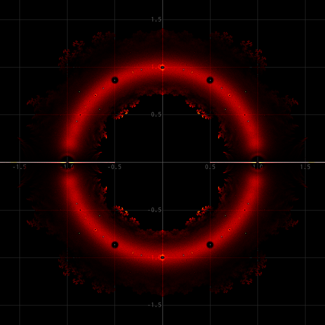
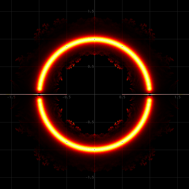
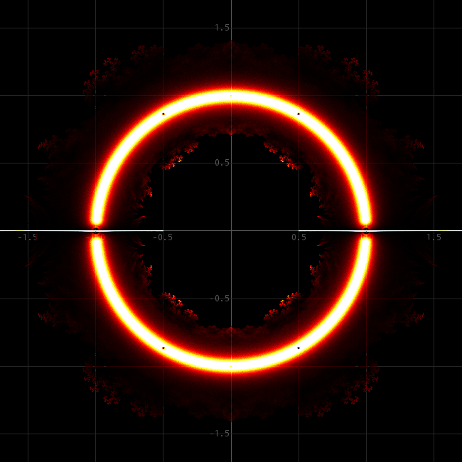
The pictures show that for increasing degree the number of very hot pixels increases. This is easy to explain, because of the fact that for an n^th degree polynomial the total number of roots equals 2000000n. So, for higher n there are more roots to be used to make hot pixels.

What, however, is very peculiar is that further away from the unit circle |z|=1 there are interesting fractal patterns and these are (at the resolution of these images) the same for all four images. The density of zeros (the temperature of the pixels) is much higher for 50^th degree polynomials close to the unit cicrle, but further away from the unit circle, the density of zeros seems to be independent of the degree of the polynomial. This is remarkable. Intuitively, one would expect the density of zeros to be larger everywhere. But even more remarkable is that for the higher degree polynomials not only the density is the same further away from the unit circle, but also their distribution of roots over the complex plane is VERY close for different degrees.
Apparently, the zeros of polynomials with coefficients taken randomly from {

back to top of page

back to main experiments page